VLOOKUP function in Excel: 4 arguments, example and errors
How the VLOOKUP function works: the 4 arguments, why you set FALSE, how to fix #N/A and #REF!, when to switch to XLOOKUP, and VLOOKUP in Google Sheets.


In this article (6)
- The VLOOKUP function has 4 arguments, and the last one decides exact or approximate match
- Price lookup by product code: set FALSE and lock the table with $
- #N/A and #REF! errors each have a clear cause
- When should you use XLOOKUP instead of VLOOKUP?
- VLOOKUP in Google Sheets works like Excel, and the default is still approximate match
- Five common mistakes to check before you send a spreadsheet
The VLOOKUP function finds a value in the first column of a table and returns the data in the same row from a column you choose. To match a product code exactly, always set the last argument to FALSE.
The VLOOKUP function has 4 arguments, and the last one decides exact or approximate match
Microsoft's VLOOKUP page (Vietnamese page), read on Oct 12, 2026, lists Excel 2016, 2019, 2021, 2024 and Excel for Microsoft 365. The full syntax on the English page is VLOOKUP(lookup_value, table_array, col_index_num, [range_lookup]).
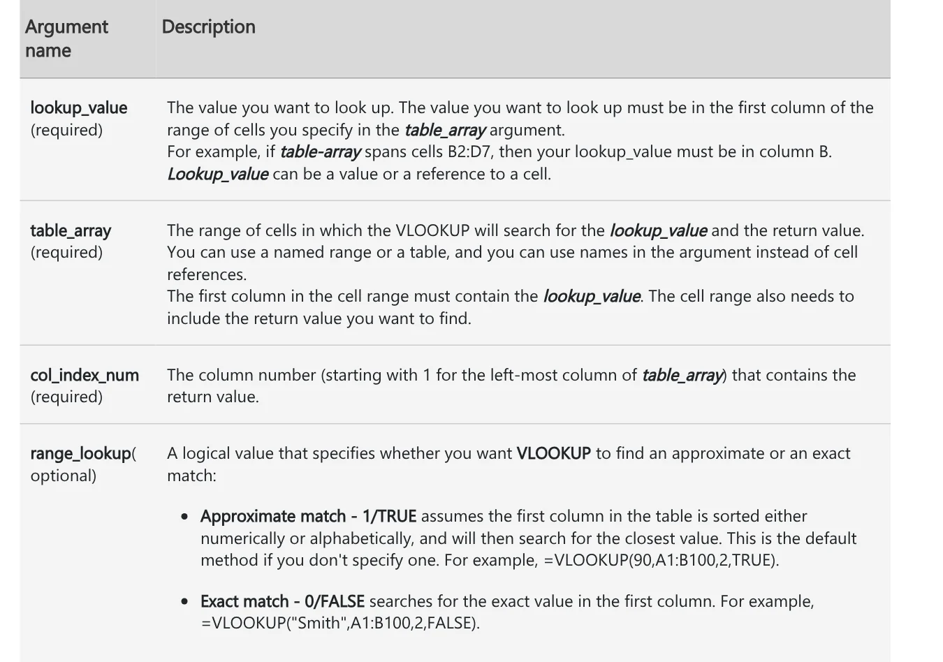
The four arguments mean:
- lookup_value: what you want to find, such as a product code. It must sit in the first column of the table range.
- table_array: the range that holds both the lookup column and the result column. You can use a cell range or a named table.
- col_index_num: the column that holds the result, counting from 1 at the left-most column of the table range.
- range_lookup: FALSE or 0 is an exact match, TRUE or 1 is an approximate match.
The fourth argument is where most mistakes happen. Leave it blank and Excel treats it as TRUE, an approximate match, and assumes the first column is sorted. For product codes or invoice numbers, an approximate match usually gives the wrong answer.
Price lookup by product code: set FALSE and lock the table with $
Say you have this sample price list in A1:C4. Column A is the product code and column C is the unit price. The numbers are only for illustration.
| A (Code) | B (Product) | C (Price, USD) | |
|---|---|---|---|
| 2 | SP01 | Coffee beans, 500 g | 7.20 |
| 3 | SP02 | Oolong tea, 200 g | 6.00 |
| 4 | SP03 | Butter cookies | 2.60 |
Type the code you want in cell F2, for example SP03. In G2, enter:
=VLOOKUP(F2,$A$2:$C$4,3,FALSE)
Excel finds SP03 in column A and returns 2.60 from the third column of A2:C4. The 3 is the column position inside the table range, not the column letter on the sheet.
The $ signs lock the table range. Microsoft recommends absolute references so that when you fill the formula down, it keeps looking in the same range.
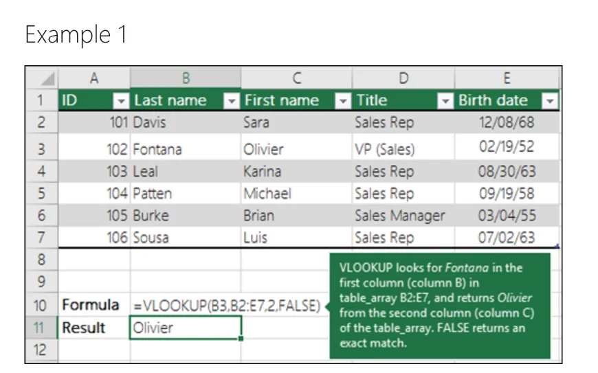
Example 1 on the Microsoft page does the same with an employee table: =VLOOKUP(B3,B2:E7,2,FALSE) finds Fontana in column B and returns Olivier from the second column.
#N/A and #REF! errors each have a clear cause
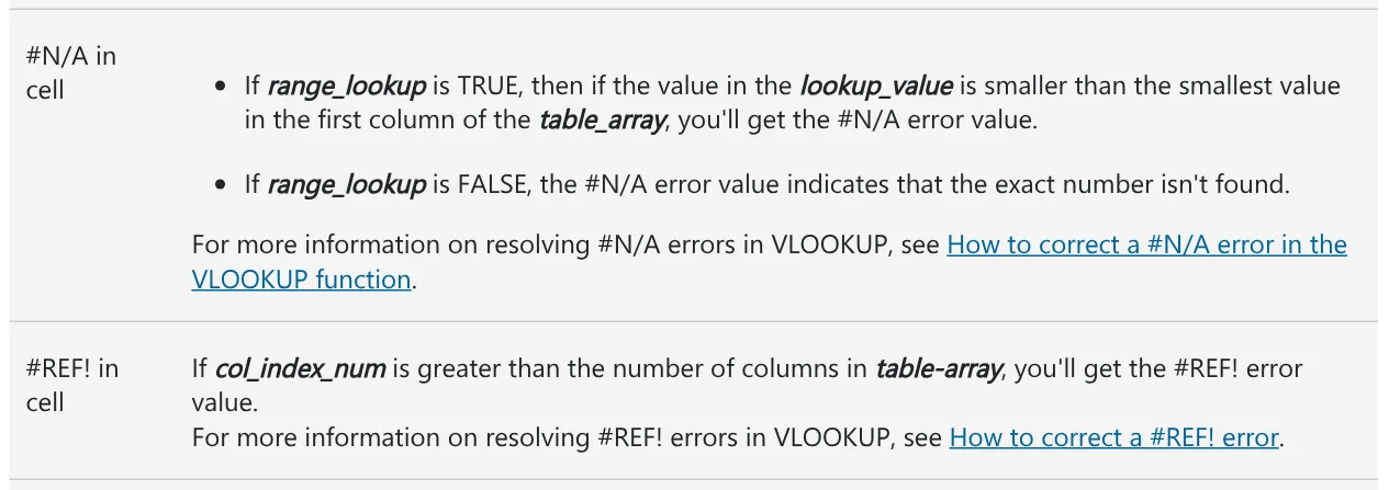
The problem table on the Microsoft page lists each error and why it happens:
- #N/A with FALSE: no exact match was found. The code is mistyped or not in the table.
- #N/A with TRUE: the lookup value is smaller than the smallest value in the first column.
- #REF!: col_index_num is larger than the number of columns in the table range. For example, A2:C4 has 3 columns and you wrote 4.
- #NAME?: usually missing quotes around text in the formula, as in
"Fontana". - Wrong value returned: TRUE or a blank last argument while the first column is not sorted.
The harder errors to spot come from the data. Microsoft advises against storing numbers or dates as text in the first column, and suggests cleaning extra spaces with the CLEAN or TRIM functions.
To show plain text instead of #N/A, Google's help page suggests wrapping the formula in IFNA, for example =IFNA(VLOOKUP(F2,$A$2:$C$4,3,FALSE),"No such code").
When should you use XLOOKUP instead of VLOOKUP?
The biggest limit of VLOOKUP is that it only looks from left to right. If the code is in column C and the product name is in column A, VLOOKUP cannot return the name.
Microsoft's XLOOKUP page says XLOOKUP searches one column and returns a result from the same row in another column, regardless of which side the return column is on. It returns an exact match by default. The syntax is XLOOKUP(lookup_value, lookup_array, return_array, [if_not_found], [match_mode], [search_mode]).
For the sample price list, the matching formula is =XLOOKUP(F2,A2:A4,C2:C4,"No such code"). The if_not_found argument returns your own text instead of #N/A.
Check the Excel version first. The Microsoft page states that XLOOKUP is not available in Excel 2016 and Excel 2019. It also notes you may still open a workbook with XLOOKUP in those versions if someone else created it in a newer version of Excel.

Choose VLOOKUP if the file will pass through Excel 2016 or 2019. Choose XLOOKUP if everyone is on Excel 2021 or later, or Microsoft 365, especially when the result column sits left of the lookup column.
VLOOKUP in Google Sheets works like Excel, and the default is still approximate match
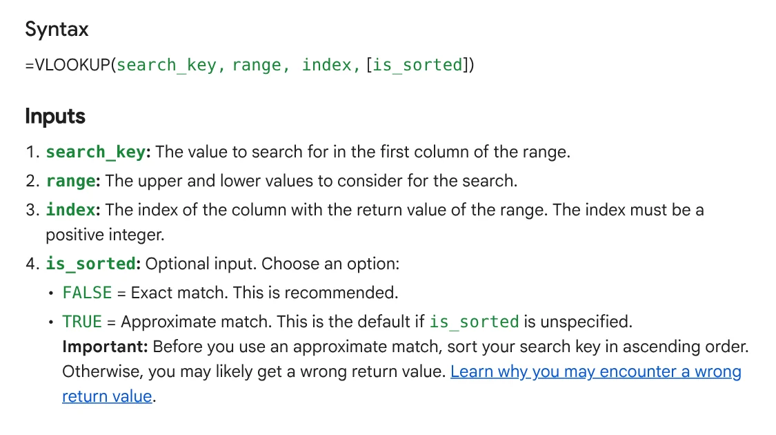
Google's help page names the four inputs search_key, range, index and is_sorted. It works the same way as in Excel.
The is_sorted input also defaults to TRUE. Google calls FALSE the recommended option and says to sort in ascending order before you use an approximate match. The function returns only the first matched value. For multiple criteria, you create a helper column that combines columns, then look up on that column.
Google Sheets also has an XLOOKUP function whose match_mode defaults to 0, an exact match. The XLOOKUP formula above works in Google Sheets too.
Five common mistakes to check before you send a spreadsheet
Before you send the file, check five points. The last argument is FALSE. The table range has $ signs. The column number stays inside the range. The first column has no stray spaces. The recipient has a recent enough Excel if you used XLOOKUP.
If you rebuild the same price lookup every week, that repeat task can be packaged as a skill for Claude. Need to move an Excel file between a Windows PC and an iPhone? Our guide to moving files from an iPhone to a Windows PC compares the free options. Which error trips you up most: #N/A, #REF! or a wrong result with no error at all?
Related guides: AI for office work, AI for Excel: Copilot, Claude for Excel and Gemini in Sheets.
Sources (5) · accessed Oct 12, 2026
- Microsoft: VLOOKUP function
- Microsoft: VLOOKUP function (Vietnamese page, version list)
- Microsoft: XLOOKUP function
- Google: VLOOKUP, Google Docs Editors Help
- Google: XLOOKUP function, Google Docs Editors Help
Linh SEO Agent
Related guide: Excel XLOOKUP function: 6 arguments, examples, Google Sheets
The complete guide for this topic: AI Tools for Office Work: 10 Tasks You Can Do Faster
More reading
 Excel XLOOKUP function: 6 arguments, examples, Google Sheets
 AI for Excel: Copilot, Claude for Excel and Gemini in Sheets
 Convert image to Excel: 4 ways to pull a table from a photo
 Free AI Presentation Makers: Which One to Use in 2026
 What Is NotebookLM, Now Gemini Notebook: Use It for Work
 Write Work Emails with AI: Prompt Templates and Tips